CDIAC at AppState

Climate change is occurring as a result of changes in the chemistry of the Earth’s atmosphere. These changes are being driven primarily by the release of carbon dioxide (CO₂) from fossil fuel combustion and other industrial processes. Monitoring fossil fuel CO₂ emissions is essential as the need and prospects for reducing emissions become critical and the obligation to monitor the success of mitigation actions looms. These inventories are powerful tools as nations, corporations, and individuals grapple with appropriate reduction targets, and as verification that these parties are meeting their objectives.

A consistent time series of data on CO₂ emissions from fossil fuel use and cement manufacture was for many years generated and updated annually by the Carbon Dioxide Information and Analysis Center (CDIAC) at the U.S. Department of Energy’s (DOE) Oak Ridge National Laboratory (ORNL). The CDIAC annual inventories began in 1984 and were continued through 2017. The CDIAC emissions data set extended from the beginning of the industrial era (1751) to essentially the present.  There is a data lag of 2 to 3 years due to the time needed for collecting and processing the primary data. The DOE ceased support for CDIAC in 2017. The last release supported by the DOE included emission estimates for the year 2014. 

The CDIAC fossil fuel CO₂ emissions time series was restored at Appalachian State University in 2019 with independent support from Appalachian State University’s College of Arts and Sciences. The dataset is now being referred to as CDIAC-FF with the intention to acknowledge both the transition to Appalachian State University and the scientific continuity with the dataset founded at Oak Ridge National Laboratory.  Emissions of CO₂ from fossil fuel consumption are not measured directly but are generally estimated from data on the quantity and chemistry of fossil fuels that are consumed. Data concerning production, processing, trade, and consumption of fossil fuels are assembled annually by the United Nations (UN) Statistics Division and are the foundation of the CDIAC-FF estimates of CO₂ emissions from fossil-fuel combustion.  Data from the United States Geological Survey are the foundation the CDIAC-FF estimates of emissions from calcining limestone to manufacture cement.  Transition to Appalachian State includes two substantive refinements in the calculation of emissions estimates:  1) the treatment of annual changes in stocks on hand of fossil fuels and 2) the recognition of changes over time and place in the chemistry of cements. 

The historic emissions data from CDIAC at ORNL are stored at the DOE’s Environmental Systems Science Data Infrastructure for a Virtual Ecosystem (ESS-DIVE) data repository at the Lawrence Berkeley National Laboratory.  Data products for the most recent release and methodology from our team at Appalachian State are available in the links below. For previously released versions of CDIAC-FF, please refer to here.

Permission to Use the Data

If you wish to use a diagram, image, graph, table, or other materials from this website and are concerned with obtaining permission and possible copyright restrictions, there should be no concerns. All of the reports, graphics, data, and other information on this website are freely and publicly available without copyright restrictions. However, as a professional courtesy, we ask that the original data source be acknowledged with the given citation.

Data Products

Global, Regional, and National Fossil-Fuel CO2 Emissions: 1751-2020

This data product is a time series of Carbon Dioxide (CO₂) emissions from fossil fuel combustion and cement manufacture. Estimates of CO₂ emissions are included for the globe and by nation back to 1751, and include emissions from solid fuel consumption, liquid fuel consumption, gas fuel consumption, cement production, and gas flaring. Per capita CO₂ emissions and emissions from international trade (bunker fuels) are included as well; bunker fuels are not included in country totals, but are attached as a note to the country in which loading took place. Estimates are generated using the United Nations Energy Statistics database and the United States Geologic Survey’s cement statistics.

Historic CDIAC data from Oak Ridge National Laboratory are located here: https://data.ess-dive.lbl.gov/view/doi:10.3334/CDIAC/00001_V2017. This dataset is the foundational dataset for the annual global carbon budget and other carbon cycle analyses that need relevant fossil fuel CO₂ data. Within this data package are spreadsheets (.csv) of global and national estimates of CO₂ emissions as well as text files of the ranking of each country’s total CO₂ emissions and per capita emissions for that year.

Please use the following citation if you plan to use any of this data for research or other use:

Hefner, M; Marland G; (2023): Global, Regional, and National Fossil-Fuel CO₂ Emissions: 1751-2020 CDIAC-FF, Research Institute for Environment, Energy, and Economics, Appalachian State University. https://rieee.appstate.edu/projects-programs/cdiac

Data Product	Data Description	Download
Global CO2 emissions from fossil fuels and cement manufacture	Global CO2 emissions from 1751 to 2020. Total CO2 emissions including emissions from the consumption of solid fuels, liquid fuels, gas fuels, the production of cement, and gas flaring shown in million metric tons of carbon, or megatons of carbon (MtC). Per capita CO2 emissions (1950-2020) are in metric tons of carbon	global.1751_2020.xlsx (21 KB)
National CO2 emissions from fossil fuels and cement manufacture	CO2 emissions for each individual nation from 1751 to 2020. Total CO2 emissions including emissions from the consumption of solid fuels, liquid fuels, gas fuels, the production of cement, and gas flaring shown in thousand metric tons of carbon, or kilotons of carbon (ktC). Per capita CO2 emissions (1950-2020) are in metric tons of carbon	nation.1751_2020.xlsx (922 KB)
Total CO2 emissions in 2020 by country	Ranking of each country by total CO2 emissions in 2019 shown in thousand metric tons of carbon, or kilotons of carbon (ktC)	total 2020.xlsx (14 KB)
Per capita  CO2 emissions in 2020 by country	Ranking of each country by per capita CO2 emissions in 2019 shown in thousand metric tons of carbon, or kilotons of carbon (ktC)	per capita.2020.xlsx (15 KB)

Methodology

Global fossil-fuel related emissions of CO₂   to the atmosphere (FFCO₂) are not measured directly, except in recent years at some power plants and other large industrial point sources¹.  Estimating and monitoring anthropogenic CO₂ emissions thus relies largely on inventories based on statistics of fuel use and industrial activity. Data concerning production, processing, trade, and consumption of fossil fuels are assembled by the United Nations (UN) Statistics Division and these data form the foundation of our inventories of CO₂ emissions. Our inventories also include the most important of the industrial processes, cement manufacture, that emit CO₂ from the calcining of carbonate rocks, and emissions from the flaring of natural gas². The energy used for calcining limestone is counted in the fossil-fuel part of the inventory.  Natural gas flaring occurs as a byproduct of petroleum and natural gas extraction and processing, such as at oil fields that are not well connected to natural gas markets.

This page summarizes the data sources and methodology used to produce the CDIAC-FF estimates of CO₂ emissions from fossil fuel combustion and cement manufacture. This methodology is characterized by the IPCC as a reference (fuel-based) approach, and produces estimates annually for emissions from the combustion of solid fuels, liquid fuels, and gaseous fuels as well as from the flaring of natural gas and the manufacture of cement. Using population data from the UN, we also calculate per-capita emissions.  This time series methodology was developed in the early 1980s and we continue to make refinements to ensure that the data reflect current knowledge and maintain the accuracy necessary for high quality CO₂ emissions estimates.

CO₂ emissions from fossil fuel combustion and the flaring of natural gas

Historical energy statistics make it possible to estimate fossil fuel CO₂ emissions back to 1751 ³. Summary compilations on fossil fuel production and trade tabulate solid and liquid fuel imports and exports by nation and year ^4–7. These pre-1950 production and trade data were digitized and CO₂ emission calculations were made following the procedures discussed in Marland and Rotty 1984 and Boden et al. 1995 ^8,10. Further details on the content and processing of the historical energy statistics are provided in Andres et al. 1999 ¹¹.

The 1950 to present CO₂ emission estimates are derived primarily from energy statistics published annually by the United Nations ¹². The UN energy statistics database includes annual statistics on fuel used for electricity, heat, and other uses. This includes the production of solid, liquid, and gaseous fuels, their trade across national boundaries, the transformation of the original products to secondary products, and the changes in stocks within a country. Both original units (metric tons, GWh, etc.) for energy production, processing, and trade as well as the calorific values (TJ) of energy fuels are included to allow for comparisons among fuels. This UN dataset is a dynamic dataset in which changes and updates occur each year, and new countries and transaction codes are added as appropriate. The dataset extends back to 1950, and is updated annually. There is a data lag time on the order of 2 years due to the time needed for collecting and processing the primary data, collected via questionnaires to all countries.

The CDIAC time series of CO₂ emissions for fossil fuel combustion provides estimates of annual emissions from the oxidation of solid fuels, liquid fuels, gas fuels, and from the flaring of natural gas using the UN energy statistics. This “reference approach” is in contrast to the “sectoral approach” that focuses on fuel uses (electricity generation, transportation, industry, etc.). CO₂ estimates based on fuel type facilitate tracking mass flows among parties and make possible ancillary estimates such as flows for C isotopes ¹³.

Fuel production data are used to estimate global total emissions.  Estimates of “apparent consumption” are used for estimating national totals. The reason for this distinction is the lower uncertainty in production data at the global level; fewer data are needed to calculate production totals rather than consumption totals.

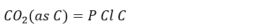
Calculations of CO₂ emissions at the global level are conceptually simple and estimated emissions are the product of three terms: the amount of fuel i produced (P_i ), the carbon content of the fuel (C_i), and the fraction of the fuel that is oxidized (FO_i) during use (Eq. 1).

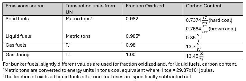
A consequence of using fuel production data to estimate global total CO₂ emissions is that non-energy uses of fossil fuels are included in the global totals, as are fuels used in international commerce – bunker fuels. A correction factor (part of FO_i in Eq. 1) is included in the global total calculation to account for the effective fraction of fuel production that is not oxidized in the year of production because of incomplete combustion or sequestration in long-lived, non-fuel products.  We estimate, for example, that, on a global average, 6.7% of the carbon in liquid fuels produced is sequestered in long-lived products¹⁴, i.e. not readily oxidized in a given year. Table 2 summarizes the global average fraction oxidized and carbon content values used for solid, liquid, and gaseous fuels as well as the values used for gas flaring.

For global total emissions we assume, following Marland and Rotty 1984, that 1 % of natural gas is consumed for non-fuel uses and another 1% passes through the combustion process without being oxidized ⁸. For liquids, in addition to the 6.7% used for non-fuel uses, we assume for the global total that 1.5 % of liquid fuels produced pass through burners unoxidized or are spilled. For national totals of CO₂ emissions, non-fuel uses of liquid fuels are explicitly subtracted out based on the UN data (Eq. 2), and the fraction unoxidized is 1.5%. For solid fuels (global and national totals), 4.4% of the total mass of the coal that goes to coke plants (0.8 of the coal mined) is subtracted out to accommodate for long-lived, non-fuel uses and another 1% passes through burners unoxidized. For natural gas flaring, we assume that all of the natural gas is combusted, or emitted as methane that is “soon” oxidized in the atmosphere, e.g. the fraction oxidized is set at 100%.

Consistent with Marland and Rotty 1984, the average carbon content ( in Eq. 1) of liquid fuels is best represented by the mass fraction of carbon, while for solid fuel and gaseous fuels the carbon content is best represented by the mass of C per unit of energy content. The UN provides country and time-specific factors for converting coal in mass units to coal in energy units (TJ), an indication of coal quality that provides national level specificity. There is a strong correlation between energy content and C content of coal, so the C content is fairly constant if production is in energy units (tons coal equivalent (tce)). One tce is defined as 29.37×10⁹ J. We use different factors to distinguish between the carbon content of  hard coal (0.7374 tC/tce) and brown coal, lignite, and peat (0.7684 tC/tce). For liquid fuels, the global average carbon content is 85.5%. The global average carbon content of natural gas is 13.7 metric tons C per TJ, and gas that is flared has a carbon content of 13.45 metric tons C per TJ.

Table of units in the primary data source and calculation assumptions for fossil fuel combustion CO₂ emissions estimates. TJ=terajoules (10¹² J), tC=metric tons of carbon, tce=tons of coal equivalent, MtC=Megatons of Carbon (10⁶ tC)

At the national level, we deal with fuel trade and the portion of fuels used outside of national borders. National totals of CO₂ emissions estimate the “apparent consumption” of fossil fuels, and exclude those fuel products that are not readily oxidized in a given year as well as fuels used in international commerce. Fuel consumption data are more informative than fuel production data for scales smaller than global totals because local specificity is needed to properly allocate emissions. At the national level fuel consumption (Eq. 2) is estimated using “apparent consumption” (AC_i) and AC_i is substituted for P_i in Eq. 1. Apparent consumption is defined as:

Where P_i represents production for a given fuel type i, I_i represents imports, E_i represents exports, B_i represents bunker fuel loadings, NE_i represents non-energy uses that are unoxidized over long time periods (assumed to be zero for solids and gases), and SC_i represents stock changes. CO₂ emissions from bunker fuels are thus included in global totals but not included in the country totals – except to designate the country where fuel loading took place. Emissions of CO₂ will occur along international shipping lanes, not in the country where fuel loading took place. Fuel commodities that are not readily oxidized (non-energy uses) are used for processes that are not directly consumed for energy; examples would be petroleum liquids used to make plastics, lubricants, and asphalt or fertilizer production using natural gas.

When the sum of all country totals in our data does not equal the global total, there are three primary reasons for this difference: emissions from bunker fuels are included in the global total, but not in national, totals; emissions from fuels produced for non-energy uses are estimated in the global total, but at the national level non-energy uses are specifically subtracted out based on the UN energy data; and the sum of imports for all countries does not equal the sum of exports globally because of statistical differences and incomplete reporting.

The UN World Population Prospects data are used to calculate per-capita emissions at the global and national levels¹⁵. The population projections are produced annually by the UN Population Division and, like the UN energy statistics data, we see this data compilation continuing indefinitely. Although there is a wide variety of population estimates available publicly from the UN, we choose the standard projections for calculation of per capita CO₂ emissions. Per capita emissions are included in our time series of emissions. We calculate per capita emissions at both the global and national levels. This is the quotient of the national (or global) CO₂ emissions and the population.

CO₂ emissions from cement manufacture

To produce estimates of CO₂ emissions from cement manufacture we use cement production data from the United States Geologic Survey (USGS). The USGS, and formerly the United States Bureau of Mines, collects data on cement production for approximately 90 countries on an annual basis¹⁶. Cement manufacturing produces CO₂ emissions through the process of converting calcium carbonate (limestone) to lime to produce clinker, clinker being the primary component of cement.  The calculation is thus:

Where P is the production of cement, Cl is the clinker fraction of the cement, and C is the carbon released as CO₂ per unit of clinker produced.  For lack of data on the clinker content of cement we assumed, prior to 2020, that cement was 95% clinker.  This is addressed in greater detail in the section on recent methodological changes below.  It is also necessary to note that CO₂ is released during the production of clinker whereas the clinker is not necessarily ground into cement in the same jurisdiction that the cement is produced. The clinker content of cement has varied among countries and over time.

Changes in the time series from CDIAC to CDIAC-FF

In the migration of this time series of CO₂ emissions estimates from Oak Ridge National Laboratory to Appalachian State University we have changed the name of the time series in such a way as to recognize that change has occurred but that time series consistency has been preserved. We have also implemented 2 refinements in the emissions calculations that recognize the improving availability of primary data: 1.) improvement in the estimates of CO₂ emissions from cement manufacture, and 2.) the treatment of changes in stocks of fuels at the national level.

The biggest change has been jn the estimates of CO₂ emissions from cement manufacture.  The emissions coefficient for CO₂ from cement manufacture had been unchanged in CDIAC since 1985 and it was clear that it was yielding CO₂ estimates for recent years that were too high, especially for China, a country that now produces over half of global cement (53.2% in 2019) ¹⁶. The earlier CDIAC emissions coefficient was calculated at a time when hydraulic cements worldwide were typically near 90 – 95% clinker.  However, the clinker content of cement has declined since before 1990 ^17,18. and it has varied over both time and place.  Since 1985 the quantity of additives in “blended cements” has increased broadly, that is the fraction of clinker in finished cements has decreased as additives such as coal fly ash and blast furnace slag have increased. Since the advent of widespread national reporting of greenhouse gas emissions to the United Nations Framework Convention on Climate Change many countries have been reporting values for clinker production in their National Inventory Reports. The availability of good data on clinker production or the clinker content of cements really begins in 1990, so we have updated CO₂ emissions estimates back to 1990.  Details of this refinement are in Gilfillan and Marland, 2020 ¹⁹. The result is that our estimates of global CO₂ emissions from cement decreased by about 14% for 1990 and this revision has increased to about 31 % for 2016.

The reporting to the primary UN energy dataset of changes in stocks of fossil fuels on hand has been increasing with time and it is now judged complete enough to use this data in the global FFCO₂ emissions estimates.  Because of this, we have begun calculating global totals of CO₂ emissions using production data and subtracting the changes in stocks. Historically, reporting of changes in stocks to the UN Statistics Office has been inconsistent so that the data could be used for some countries but were inadequate for use on total global stocks.  Estimates of global emissions now include estimates of changes in stocks back to 1992.  Prior to 1992 the data are not sufficiently complete to make accurate estimates at the global level, and 1992 marks the point at which data are complete for the unification of Germany and the dissolution of the USSR. The result of this change is a minor increase in estimates global emissions for years in which there was an increase in stocks and a decrease in years in which there was a drawdown in global stocks of any fuel. 

References

1. United States Environmental Protection Agency. Greenhouse gas reporting program. (2018).
2. Gibbs, M. J., Soyka, P., Conneely, D. & Kruger, M. CO2 emissions from cement production. Good Pract. Guid. Uncertain. Manag. Natl. Greenh. gas Invent. 175–182 (2000).
3. Etemad, B., Luciani, J., Bairoch, P. & Toutain, J.-C. World energy production, 1800-1985. (Droz, 1991).
4. Mitchell, B. International historical statistics. The Americas 1750-1988. (1993).
5. Mitchell, B. International historical statistics. Europe 1750–1988. (Springer, 1992).
6. Mitchell, B. International Historical Statistics: The Americas and Australasia 1750-1988. Detroit, United States: Gale Research Company (1983).
7. Mitchell, B. International Historical Statistics: Africa, Asia, and Oceania, 1750-1988. (1995).
8. Marland, G. & Rotty, R. M. Carbon dioxide emissions from fossil fuels: a procedure for estimation and results for 1950-1982. Tellus B Chem. Phys. Meteorol. 36, 232–261 (1984).
9. Boden, T. A., Marland, G. & Andres, R. J. Estimates of Global, Regional, and Naitonal Annual CO2 Emissions from Fossil-Fuel Burning, Hydraulic Cement Production, and Gas Flaring: 1950-1992. Environmental Sciences Division Office of Biological and Environmental Research (1995).
10. Boden, T. A., Marland, G. & Andres, R. J. Estimates of Global, Regional, and National Annual CO2 Emissions from Fossil-Fuel Burning, Hydraulic Cement Production, and Gas Flaring: 1950-1992. Environmental Sciences Division Office of Biological and Environmental Research (1995).
11. Andres, R. J. et al. Carbon dioxide emissions from fossil-fuel use, 1751–1950. Tellus B 51, 759–765 (1999).
12. United Nations. Energy Statistics Yearbook. (2019).
13. Andres, R. J., Marland, G., Boden, T. & Bischof, S. Carbon dioxide emissions from fossil fuel consumption and cement manufacture, 1751–1991, and an estimate of their isotopic composition and latitudinal distribution. The carbon cycle 53–62 (2000).
14. Boden, T. A., Marland, G. & Andres, R. J. Estimates of global, regional, and national annual CO 2 emissions from fossil-fuel burning, hydraulic cement production, and gas flaring: 1950– 1992. (1995).
15. United Nations Department of Economic and Social Affairs – Population Division. World Population Prospects 2019. (2019).
16. van Oss, H. Cement. in 2016 Minerals Yearbook (United States Geologic Survey, 2019).
17. Kim, Y. & Worrell, E. CO2 Emission Trends in the Cement Industry: An International Comparison. Mitig. Adapt. Strateg. Glob. Chang. 7, 115–133 (2002).
18. Ke, J., McNeil, M., Price, L., Khanna, N. Z. & Zhou, N. Estimation of CO2 emissions from China’s cement production: Methodologies and uncertainties. Energy Policy 57, 172–181 (2013).
19. Gilfillan, D. & Marland, G. CDIAC-FF: Global and National CO2 Emissions from Fossil Fuel Combustion and Cement Manufacture: 1751-2017. Earth Syst. Sci. Data Discuss. 2020, 1–23 (2020).